Modules over Principal Ideal Domains (pdf)

We present the fundamental structure theorems for modules over principal ideal domains and provide a selection of their applications. In particular, we show how the Smith Normal Form and the Jordan Normal Form can be derived from these structure theorems.

1. Introduction

Modules over rings are often introduced as a generalization of vector spaces and it is therefore tempting to think of modules in the same way as vector spaces. However, the following pathological example will illustrate that the intuition that we have built up during studying vector spaces is in general not applicable to modules.

Consider the ring $R=\mathbb{Z}[\sqrt{-5}]$ and the ideal $I=(2,1+\sqrt{-5})$. Then $I$ defines a $R$-module and as such $I$ is finitely generated by the set $\{2,1+\sqrt{-5}\}$. But

$$\begin{array}{r}(1+\sqrt{-5})\cdot 2+(-2)\cdot (1+\sqrt{-5})=0\end{array}$$

shows that these elements are not linearly independent. In fact, by an analogous choice of coefficients any two elements $x,y$ of $I$ are linearly dependent. On the other hand, one can show that $I$ is not principal, i.e. there is no single element that generates $I$ (one way to do this is by considering the field norm $N(a+b\sqrt{-5})=a^2+5b^2$). This example illustrates a key difference between modules and vector spaces. Namely, if a vector space contains a finite spanning set, then it contains a finite basis. This example shows that this is in general not true for modules. Furthermore, we notice that even though $R$ (viewed as an $R$-module) is free of rank one, the submodule $I$ is not free and is something in-between the zero-module and $R$. Again this cannot happen in a vector space. If we consider a vector space of dimension one, then the only subspaces are the zero space and the whole space itself.

Remarkably, if we restrict our attention to modules over principal ideal domains, their structure becomes significantly more regular. The rest of this text will be concerned with exploring this well-behaved structure of modules over principal ideal domains and discuss some of its consequences.

In what follows, we assume that the reader is familiar with Ring Theory and the very basics of module theory. However, we do not assume any prior knowledge about modules over principal ideal domains.

2. Structure Theorems

Our first important theorem asserts that if we consider a submodule of a freely generated module over a principal ideal domain, then we cannot end up as in the example provided in the introduction, i.e. the submodule will always be freely generated as well.

We fix a principal ideal domain $R$ for the remainder of this section.

Theorem 1

Let $F$ be a free module of finite rank over $R$ and $M$ a submodule. Then $M$ is free of rank less than or equal to the rank of $F$.

Proof:
Let $e_1,\dots ,e_n$ be a basis of $F$ over $R$. Set

$$M_r=M\cap \underset{i=1}{\overset{r}{⨁}}R{e}_i,$$

for $r=0,\dots ,n$, where the empty sum is defined as the zero module. We now prove by induction on $r$, that each $M_r$ is finitely generated with rank $\le r$. The zero-module is free of rank zero, hence the statement holds for $r=0$. Now assume that the statement holds for $0\le r<n$. Let $p:F\to R$ be the projection to the $(r+1)$‘th coordinate, i.e. the linear continuation of

$$p(e_i)=\{\begin{array}{ll}1& i=r+1\\ 0& \text{otherwise}.\end{array}$$

for $i=1,\dots ,n$. Then $p$ defines a module homomorphism and hence $p(M_{r+1})$ is a submodule of $R$, i.e. an ideal. We now use the fact that $R$ is a principal ideal domain to obtain a generator $\alpha$ of $p(M_{r+1})$. If $\alpha =0$, then by construction $M_r=M_{r+1}$ and we are done with the induction step. Otherwise, choose $v\in p^{-1}(\alpha )$. We claim that $M_{r+1}=M_r\oplus Rv$, which would imply that $M_{r+1}$ is free of rank $\le r+1$. Indeed, let $x\in M_{r+1}$. Then $p(x)\in R\alpha$, hence there exists a $b\in R$ such that $p(x-bv)=0$. This shows that $M_{r+1}=M_r+Rv$. Furthermore, if $x\in M_r\cap Rv$, then $x=bv$ for some $b\in R$. But since $p(M_r)=\left\{0\right\}$, we have $p(x)=b\alpha =0$, hence $b=0$, which implies $x=0$. This shows that the sum is direct and thus concludes the proof.

$$\begin{array}{r}\end{array}\text{\hspace{1em}□}$$

Remark 2

Using the axiom of choice one can prove this theorem without the assumption that $F$ has finite rank, see (Rotman, 2015).

Next, we will proof another key theorem in the theory of modules over principal ideal domains. It is essentially a statement about finding aligned bases of a module and a submodule, as we will illustrate after we give the proof.

Theorem 3

Let $F$ be a free module over $R$, and let $M$ be a finitely generated submodule. Then there exists a basis $\mathcal{B}$ of $F$, elements $e_1,\dots ,e_n\in \mathcal{B}$, and non-zero elements $a_1,\dots ,a_n\in R$ such that

$$\begin{array}{r}M=\underset{i=1}{\overset{n}{⨁}}R{a}_i{e}_i,\end{array}$$

and $a_1|a_2|\dots |a_n$.

Proof:
We first notice that given a basis of $F$, we can write each generator of $M$ as linear combinations of finitely many elements of said basis. Since $M$ is finitely generated, we obtain a finite set of linearly independent elements of $F$ that generate a free submodule $F^{\prime }$ such that $M\subseteq F^{\prime }\subseteq F$. We can thus assume without loss of generality that $F$ has finite rank.

We note that in the case where $F$ or $M$ is the zero-module the theorem holds trivially. We may thus assume for a smoother argument that neither $F$ nor $M$ is the zero-module.

To begin, let us consider the set of ideals

$$\begin{array}{r}\{\phi (M):\phi \in {\mathrm{Hom}}_R(F,R)\}.\end{array}$$

Since $R$ is a principal ideal domain, the above set contains a maximal element under inclusion, say $\lambda (M)$ for $\lambda \in {\mathrm{Hom}}_R(F,R)$ (see Lemma A2 for details). Again using the fact that $R$ is a principal ideal domain we find an $a_1\in R$ such that $\lambda (M)=(a_1)$. Let $x_1\in M$ be such that $\lambda (x_1)=a_1$. We claim that for any $\phi \in {\mathrm{Hom}}_R(F,R)$ we have $\phi (x_1)\in (a_1)$. Indeed, let $d\in R$ be a greatest common divisor of $\phi (x_1)$ and $a_1$ and let $\alpha ,\beta \in R$ be such that $d=\alpha \phi (x_1)+\beta a_1$ (this is possible since $R$ is a principal ideal domain). By construction we have $(a_1)\subseteq (d)\subseteq (\alpha \phi +\beta \lambda )(M)$ and now maximality of $(a_1)=\lambda (M)$ implies $(a_1)=(d)$. This shows that $a_1$ is a divisor of $\phi (x_1)$ and hence $\phi (x_1)\in (a_1)$, as claimed. Finally, we note that the assumption that $M$ is not the zero-module implies that $a_1\ne 0$.

Let $v_1,\dots ,v_n$ be a basis of $F$ and write $x_1={\alpha }_1{v}_1+\cdots +{\alpha }_n{v}_n$ with ${\alpha }_i\in R$ for all $i$. By considering the functionals given by the projections onto the $i$‘th coordinate with respect to the basis $v_1,\dots ,v_n$, we obtain with the conclusion of the previous paragraph that $a_1|{\alpha }_i$ for all $i$. Thus, there exists an element $e_1\in F$ such that $x_1=a_1{e}_1$. Finally, we notice that linearity of $\lambda$ together with $a_1\ne 0$ imply that $\lambda (e_1)=1$.

We now claim that $F$ may be decomposed in to the direct sum

$$\begin{array}{r}F=R{e}_1\oplus \ker \lambda .\end{array}$$

Indeed, let $v\in F$, then

$$\begin{array}{r}\lambda (v-\lambda (v)e_1)=\lambda (v)-\lambda (v)\lambda (e_1)=0,\end{array}$$

and hence $v-\lambda (v)e_1\in \ker \lambda$. This shows $F=R{e}_1+\ker \lambda$. Now, let $v\in R{e}_1\cap \ker \lambda$. Write $v=\alpha e_1$ for some $\alpha \in R$. Then, we obtain $\lambda (v)=\alpha \lambda (e_1)=0$. Since $\lambda (e_1)=1$, this yields $\alpha =0$ and so $v=0$. This shows $R{e}_1\cap \ker \lambda =\{0\}$ and thus the above decomposition into a direct sum holds. Using the fact that $\lambda (M)=(a_1)$, an analogous argument shows

$$\begin{array}{r}M=R{a}_1{e}_1\oplus (\ker \lambda \cap M).\end{array}$$

Now if $\ker \lambda \cap M$ is the zero-module we are done. Otherwise, we apply Theorem 1 to obtain that $\ker \lambda$ is again a free module of finite rank and $\ker \lambda \cap M$ a finitely generated submodule. We can thus inductively repeat the whole argument to obtain the decompositions

$$\begin{array}{r}F=F^{\prime }\oplus \underset{i=1}{\overset{n}{⨁}}R{e}_i,\text{and}M=\underset{i=1}{\overset{n}{⨁}}R{a}_i{e}_i,\end{array}$$

where $F^{\prime }$ is a possibly trivial free submodule of $F$. Finally, we claim that this construction yields $a_1|a_2|\dots |a_n$, without any further modifications. Indeed, let ${\pi }_i$ denote the projection of $F$ onto the coordinate of $e_i$ and consider the functional $\phi ={\pi }_1+{\pi }_2$. Then $\phi (a_1{e}_1)=a_1$ and hence $(a_1)\subseteq \phi (M)$. But by maximality of $(a_1)$ we have $(a_1)=\phi (M)$. We now obtain $\phi (a_2{e}_2)=a_2\in (a_1)$, i.e. $a_1|a_2$. Once again, by repeating this argument inductively we obtain $a_1|a_2|\dots |a_n$, thus concluding the proof.

$$\begin{array}{r}\end{array}\text{\hspace{1em}□}$$

Remark 4

We note that in Theorem 3 we can always append zeros to the sequence of $a_i$‘s such that in the case where $F$ as finite rank, we have

$$\begin{array}{r}F=\underset{i=1}{\overset{n}{⨁}}R{e}_i,M=\underset{i=1}{\overset{n}{⨁}}R{a}_i{e}_i,\end{array}$$

with $a_1|a_2|\dots |a_n$.

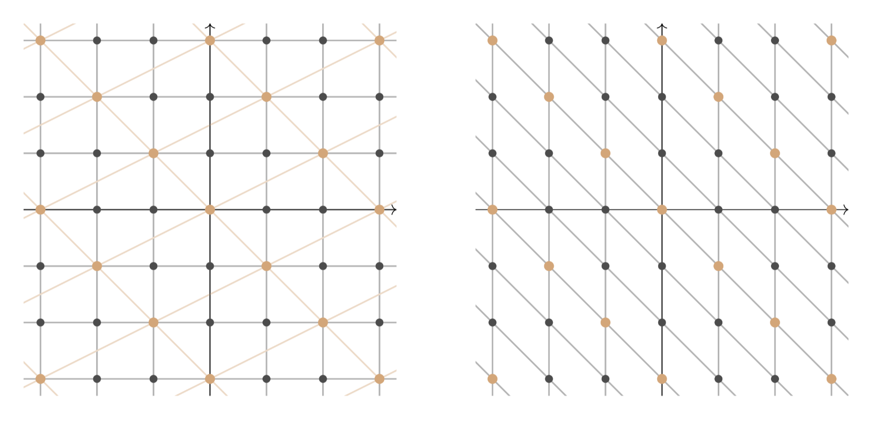
As promised, we will now provide an illustration of Theorem 3. Consider the Gaussian integers $\mathbb{Z}[i]$ viewed as a $\mathbb{Z}$-module and the submodule $M$ generated by $-1+i$ and $2+i$. If we consider the decompositions $\mathbb{Z}[i]=\mathbb{Z}\oplus \mathbb{Z}i$ and $M=\mathbb{Z}(-1+i)\oplus \mathbb{Z}(2+i)$, then these are not aligned, as the left hand side of following figure shows. However, Theorem 3 asserts the existence of aligned bases. Indeed, we find $\mathbb{Z}[i]=\mathbb{Z}(-1+i)\oplus \mathbb{Z}i$ and $M=\mathbb{Z}(-1+i)\oplus \mathbb{Z}3i$. These are visualized on the right hand side of following figure.

The following theorem builds on the previous results to give a complete classification of finitely generated modules over principal ideal domains, showing that every such module decomposes into a direct sum of a free part and cyclic torsion modules.

Theorem 5

Let $M$ be a finitely generated $R$-module. Then there exist integers $r,k\ge 0$ and element $d_1,\dots ,d_k\in R\setminus (\{0\}\cup R^{\times })$ such that

$$\begin{array}{r}M\cong R^r\oplus \underset{i=1}{\overset{k}{⨁}}R/(d_i),\end{array}$$

and $d_1|d_2|\dots |d_k$.

Proof:
Let $x_1,\dots ,x_n$ be generators of $M$. Consider the module $R^n$ and denote by $e_1,\dots ,e_n$ the standard basis of $R^n$, i.e. $e_i$ is the vector with all zeros except a one at the $i$-th entry. Now, let $\phi :R^n\to M$ be the linear map that sends $e_i$ to $x_i$ for all $i$. This map is unique and well-defined, because $e_1,\dots ,e_n$ defines a basis of $R^n$. Since $x_1,\dots ,x_n$ generate $M$, $\phi$ is surjective. Thus, by the first isomorphism theorem we have

$$\begin{array}{r}M\cong R^n/\ker \phi .\end{array}$$

Since $R^n$ is free, we may apply Theorem~\ref{thm:elementary_divisors} to obtain a basis ${\tilde{e}}_1,\dots ,{\tilde{e}}_n$ of $R^n$ and elements $a_1,\dots ,a_n\in R$ such that $\ker \phi ={⨁}_{i=1}^{n}R{a}_i{\tilde{e}}_i$ and $a_1|a_2|\dots |a_n$. We claim that

$$\begin{array}{r}{R}^n/\ker \phi \cong \underset{i=1}{\overset{n}{⨁}}R/(a_i).\end{array}$$

Indeed, consider the map

$$\begin{array}{rl}\psi :R^n=\underset{i=1}{\overset{n}{⨁}}R{\tilde{e}}_i& \to \underset{i=1}{\overset{n}{⨁}}R/(a_i)\\ \sum _{i=1}^n{x}_i{\tilde{e}}_i& \mapsto (x_1+(a_1),\dots ,x_n+(a_n)).\end{array}$$

We notice that $\psi$ defines a surjective module homomorphism. Furthermore, we note that to conclude our claim with the first isomorphism theorem we only need to show that $\ker \psi =\ker \phi$. Let $x\in R^n$ and write $x={\sum }_{i=1}^n{x}_i{\tilde{e}}_i$ for some $x_i\in R$. Then, $x\in \ker \psi$ if and only if $x_i\in (a_i)$ for all $i$, which in turn is the case if and only if $x\in \ker \phi$. This shows $\ker \psi =\ker \phi$.

Thus, by putting everything together, we obtain

$$\begin{array}{r}M\cong \underset{i=1}{\overset{n}{⨁}}R/(a_i),\end{array}$$

where $a_1|a_2|\dots |a_n$. There are now three cases of $a_i$‘s to distinguish. If $a_i$ is a unit, then $R/(a_i)$ is the zero-module, so it does not affect the direct sum and we may thus omit it in the sequence of $a_i$‘s. If $a_i$ is zero, then $R/(a_i)\cong R$. Let $r\ge 0$ be the number of zeros appearing in the sequence of $a_i$‘s. The final case to consider is if $a_i$ is a non-zero non-unit element. We collect these remaining $a_i$‘s into a sequence $d_1,\dots ,d_k$ while preserving their ordering, i.e. we still have $d_1|d_2|\dots |d_k$. Putting things together we obtain

$$\begin{array}{r}M\cong R^r\oplus \underset{i=1}{\overset{k}{⨁}}R/(d_i),\end{array}$$

thus concluding the proof.

$$\begin{array}{r}\end{array}\text{\hspace{1em}□}$$

Remark 6

We note that Theorem 5 is in essence a corollary of Theorem 3. The length of the presented proof is simply a consequence of the fairly detailed explanation of the resulting isomorphisms.

Next, we show an alternative formulation of Theorem 5 as it is sometimes more useful.

Theorem 7

Let $M$ be a finitely generated $R$-module. Then there exist integers $r,t\ge 0$, prime elements $p_1,\dots ,p_t\in R$, and integers ${\nu }_i\ge 1$ such that

$$\begin{array}{r}M\cong R^r\oplus \underset{i=1}{\overset{t}{⨁}}R/(p_i^{{\nu }_i}).\end{array}$$

Proof:
By Theorem 5 we have integers $r,k\ge 0$ and elements $d_j\in R\setminus (\{0\}\cup R^{\times })$ such that

$$\begin{array}{r}M\cong R^r\oplus \underset{j=1}{\overset{k}{⨁}}R/(d_j).\end{array}$$

Since $R$ is a principal ideal domain, there exists for each $d_j$ a unique factorization

$$\begin{array}{r}{d}_j=p_{j,1}^{{\nu }_{j,1}}\cdot \dots \cdot p_{j,s}^{{\nu }_{j,s}},\end{array}$$

where $p_{j,i}$ is prime and ${\nu }_{j,i}\ge 1$ is an integer for each $i$. Collecting all $p_{j,i}$‘s and ${\nu }_{j,i}$‘s into one sequence each, we obtain from the Chinese Remainder Theorem that

$$\begin{array}{r}\underset{i=1}{\overset{k}{⨁}}R/(d_j)\cong \underset{i=1}{\overset{t}{⨁}}R/(p_i^{{\nu }_j}),\end{array}$$

thus concluding the proof.

$$\begin{array}{r}\end{array}\text{\hspace{1em}□}$$

We conclude this section by proving that the decompositions in Theorem 5 and Theorem 7 are unique in a certain sense.

Theorem 8

The decomposition in Theorem 7 is unique up to reordering of the pairs $(p_i,{\nu }_i)$ and multiplication of the $p_i$‘s by a unit.

Proof:
Let $M$ be a finitely generated $R$-module. Then by Theorem 7, there exist integers $r,t\ge 0$, prime elements $p_1,\dots ,p_t\in R$, and integers ${\nu }_i\ge 1$ such that

$$\begin{array}{r}M\cong R^r\oplus \underset{i=1}{\overset{t}{⨁}}R/(p_i^{{\nu }_i}).\end{array}\text{\hspace{1em}(⋆)}$$

Let $p\in R$ be a prime element and $\nu \ge 0$ an integer. We notice that $p^{\nu }M/p^{\nu +1}M$ defines a module over $R/(p)$. (The action of $R/(p)$ on $p^{\nu }M/p^{\nu +1}M$ is defined by taking any representative and using the action of $R$ on $p^{\nu }M/p^{\nu +1}M$. This is well-defined because $px=0$ for any $x\in p^{\nu }M/p^{\nu +1}M$.) Hence $p^{\nu }M/p^{\nu +1}M$ defines a vector space over the field $R/(p)$. We claim that

$$\begin{array}{r}{\dim }_{R/(p)}(p^{\nu }M/p^{\nu +1}M)=r+|\{(p_i,{\nu }_i):p^{\nu +1}\mid p_i^{{\nu }_i}\}|.\end{array}$$

Assuming this claim, the theorem follows. Indeed, assume there is another decomposition of the type as in Theorem 7. We know that for vector spaces the dimension is well-defined. So by varying $p$ and $\nu$ we see that the decompositions must be the same up to reordering the pairs $(p_i,{\nu }_i)$ and multiplying the $p_i$‘s by a unit.

It thus only remains to prove the claim. To determine the dimension we note that for vector spaces we know that the dimension is preserved via isomorphisms. So it is enough to consider what happens to the right hand side of the isomorphism in $(\star )$. Consider the composition

$$\begin{array}{r}\begin{array}{ccccc}R& \to & p^{\nu }R& \to & p^{\nu }R/p^{\nu +1}R\\ x& \mapsto & p^{\nu }x& \mapsto & p^{\nu }x+(p^{\nu +1}).\end{array}\end{array}$$

Its kernel is exactly $pR$, hence $R/(p)\cong p^{\nu }R/p^{\nu +1}R$ as $R/(p)$ vector spaces. This shows that the contribution of the free part in the decomposition to the dimension of the vector space $p^{\nu }M/p^{\nu +1}M$ is exactly $r$.

Let now $(p_i,{\nu }_i)$ be a pair occurring on the right hand side of $(\star )$ such that $p^{\nu +1}\mid p_i^{{\nu }_i}$. Then we have $(p_i^{{\nu }_i})\subseteq (p^{\nu +1})$. So by the third isomorphism theorem we obtain

$$\begin{array}{r}(p^{\nu }R/(p_i^{{\nu }_i}))/(p^{\nu +1}R/(p_i^{{\nu }_i}))\cong p^{\nu }R/p^{\nu +1}R.\end{array}$$

Hence, the summand $R/(p_i^{{\nu }_i})$ contributes exactly one dimension.

Now consider a pair $(p_i,{\nu }_i)$ such that $p^{\nu +1}\nmid p_i^{{\nu }_i}$. Consider the surjective homomorphism

$$\begin{array}{rl}\phi :R/(p_i^{{\nu }_i})& \to R/(p_i^{{\nu }_i})\\ x& \mapsto p^{\nu +1}x.\end{array}$$

Then, by unique factorization in $R$ we have

$$\begin{array}{rl}\ker \phi & =\{x+(p_i^{{\nu }_i})\in R/(p_i^{{\nu }_i}):p^{\nu +1}x\in (p_i^{{\nu }_i})\}\\ & =\{x\in R:p^{\nu +1}x=p_i^{{\nu }_i}y\text{ for some }y\in R\}/(p_i^{{\nu }_i})\\ & =0+(p_i^{{\nu }_i}).\end{array}$$

Hence, $p^{\nu +1}R/(p_i^{{\nu }_i})=R/(p_i^{{\nu }_i})$ and so the quotient $(p^{\nu }R/(p_i^{{\nu }_i}))/(p^{\nu +1}R/(p_i^{{\nu }_i}))$ is the zero-module. This shows that in this case the summand $R/(p_i^{{\nu }_i})$ does not contribute to the dimension.

Putting the everything together proves the claim and thus the theorem.

$$\begin{array}{r}\end{array}\text{\hspace{1em}□}$$

Corollary 9

The decomposition in Theorem 5 is unique up to multiplication of the $d_i$‘s by a unit.

3. Applications

There are many applications of the theorems proven in Section 2. For this exposition we will focus on matrix normal forms. We begin with the so called Smith Normal Form, which in a way can be viewed as equivalent to Theorem 3, as each follows relatively quickly from the other.

Theorem 10 (Smith Normal Form)

Let $A\in {\mathrm{Mat}}_{n,m}(R)$ be a matrix. Then there exist invertible matrices $P\in {\mathrm{GL}}_n(R)$ and $Q\in {\mathrm{Mat}}_m(R)$, an integer $k\in \{1,\dots ,\min (n,m)\}$ and elements $d_1,\dots ,d_k\in R\setminus \{0\}$ with $d_1|d_2|\dots |d_k$ such that

$$\begin{array}{r}PAQ=\left(\begin{array}{cccc}{d}_1& & & \\ & \ddots & & \\ & & d_k& \\ & & & \end{array}\right),\end{array}$$

where the blank entries are zero.

Proof:
Let $N$ be the image of $A$ in $R^n$. Then $N$ is a submodule and by Theorem 3 there exists a basis $v_1,\dots ,v_n$ of $R^n$ and non-zero elements $d_1,\dots ,d_k\in R$ such that $N={⨁}_{i=1}^{k}R{d}_i{v}_i$. Let $w_i\in R$ be such that $A{w}_i=d_i{v}_i$ for each $i=1,\dots ,k$. By construction, linear independence of the $v_i$‘s implies linear independence of the ‘s. By Theorem 1, $\ker A$ is a free submodule. We claim that any basis of $\ker A$ expands the $w_i$‘s to a basis of $R^m$. Indeed, let $x\in R^m$ and write $Ax={\sum }_{i=1}^k{a}_i{v}_i$ for $a_i\in R$. Then by construction we have $x-a_i{w}_i\in \ker A$. In addition, we also have ${⨁}_{i=1}^{k}R{w}_i\cap \ker A=\{0\}$. This proves that $R^m=\ker A\oplus {⨁}_{i=1}^{k}R{w}_i$, hence our claim. In particular, there exists $w_{k+1},\dots ,w_m\in \ker A$ such that $w_1,\dots ,w_m$ defines a basis of $R^m$. We now obtain the following commuting diagram.

We see that by viewing $R^m$ and $R^n$ in the bases given by the $w_i$‘s and $v_i$‘s respectively the linear map induced by $A$ simplifies significantly. Let $Q$ denotes the change-of-basis matrix that goes from the basis $w_1,\dots ,w_m$ to the standard basis $e_1,\dots ,e_m$, i.e. $Q{w}_i=e_i$ for all $i$. Furthermore, let $P$ denote the change-of-basis matrix that goes from the standard basis $e_1,\dots ,e_n$ of $R^n$ to the basis $v_1,\dots ,v_n$, i.e. $P{e}_i=v_i$ for all $i$. Together with the commutative diagram we see that this choice of $P$ and $Q$ conclude the proof.

$$\begin{array}{r}\end{array}\text{\hspace{1em}□}$$

Next, we explore how the Jordan Normal Form arises as a consequence of the structure theorems presented in Section 2. Recall that the Jordan Normal Form is a statement about endomorphisms of vector spaces. At first glance, it may not be apparent how the theory of modules over principal ideal domains is useful in the more structured and well-behaved realm of vector spaces. The following construction will clarify this connection.

Let $V$ be a vector space over a field $K$ and $T\in {\mathrm{End}}_K(V)$ an endomorphism of $V$. Then by defining

$$\begin{array}{rl}K[X]\times V& \to V\\ (f,v)& \mapsto f(T)(v),\end{array}$$

we can view the pair $(V,T)$ as a $K[X]$-module. Conversely, let $M$ be a $K[X]$-module. Then, by restricting the multiplicative action of $K[X]$ on $M$ to $K$, we see that $M$ defines a vector space over $K$. Furthermore, if we define $T:M\to M$ via $v\mapsto X\cdot v$, then we have $T\in {\mathrm{End}}_K(M)$ and the action of $K[X]$ on $M$ is consistent with the one defined above. This construction shows that the study of pairs $(V,T)$ corresponds to the study of $K[X]$-modules.

Before we begin, a note on notation. Given a vector space $V$ over a field $K$ and an endomorphism $T\in {\mathrm{End}}_K(V)$, we will write $(V,T)$ to emphasize the $K[X]$-module structure induced by the construction above.

Lemma 11

Let $K$ be a field and let $V$ and $W$ be vector spaces over $K$. Let further $T$ and $S$ be endomorphisms of $V$ and $W$ respectively. Then $(V,T)$ and $(W,S)$ are isomorphic as $K[X]$-modules if and only if there exists a vector space isomorphism $\phi :V\to W$ such that $T={\phi }^{-1}\circ S\circ \phi$.

Proof:
We first assume that there exists a $K[X]$-module isomorphism $\phi :(V,T)\to (W,S)$. Then $\phi$ can be viewed as an isomorphism between $V$ and $W$ with the additional property that $\phi (X\cdot v)=X\cdot \phi (v)$ for all $v\in V$. This implies $\phi (Tv)=S\phi (v)$ for all $v\in V$. Hence, $T={\phi }^{-1}\circ S\circ \phi$.

Let us now assume that we have a vector space isomorphism $\phi :V\to W$ such that $T={\phi }^{-1}\circ S\circ \phi$. Then, we have $\phi (Tv)=S\phi (v)$, i.e. $\phi (X\cdot v)=X\cdot \phi (v)$ for all $v\in V$. By induction on the degree of the polynomials, we obtain that $\phi$ is $K[X]$-linear. Hence $\phi$ defines a module isomorphism between $(V,T)$ and $(W,S)$.

$$\begin{array}{r}\end{array}\text{\hspace{1em}□}$$

Lemma 12

Let $K$ be a field and $f(X)=(X-\lambda {)}^{\nu }$ for some $\lambda \in K$ and some integer $\nu \ge 1$. Consider the $K[X]$-module $K[X]/(f)$ and let $T$ be the corresponding endomorphism (according to the construction above) defined by $v\mapsto X\cdot v$. Then there exists a $K$-basis $\mathcal{B}$ of $K[X]/(f)$ such that

$$\begin{array}{r}[T{]}_{\mathcal{B}}=\left(\begin{array}{ccccc}\lambda & 1& & & \\ & \lambda & 1& & \\ & & \ddots & \ddots & \\ & & & \lambda & 1\\ & & & & \lambda \end{array}\right)\in {\mathrm{Mat}}_{\nu ,\nu }(K).\end{array}$$

Proof:
We claim that the ordered set $\mathcal{B}=((X-\lambda {)}^{\nu -1}+(f),\dots ,(X-\lambda )+(f),1+(f))$ defines a basis of $K[X]/(f)$. Indeed, we first notice that by the euclidean algorithm any equivalence class in $K[X]/(f)$ has a representative with degree $<\nu$. Thus, for an arbitrary $g+(f)\in K[X]/(f)$ we may assume that $g$ has degree $<\nu$. It is then clear that $g+(f)$ lies in the $K$ linear span of $1,X,\dots ,X^{\nu -1}$. But by considering the $K$ linear combination $g(X+\lambda )$ and substituting every $X$ with an $X-\lambda$, we see that $\mathcal{B}$ spans $K[X]/(f)$. We also find that if ${\sum }_{i=0}^{\nu -1}{a}_i(X-\lambda {)}^i=0$ for some $a_i$‘s in $K$, then by comparing coefficients starting with $a_{\nu -1}$ we find that $a_i=0$ for all $i$. This shows that $\mathcal{B}$ defines a $K$-basis of $K[X]/(f)$. We now notice that

$$\begin{array}{rl}(T-\lambda )((X-\lambda {)}^i+(f)))& =(X-\lambda )\cdot (X-\lambda {)}^i+(f)\\ & =(X-\lambda )\cdot (X-\lambda {)}^i+(f)\\ & =(X-\lambda {)}^{i+1}+(f),\end{array}$$

for all $i=0,\dots ,\nu -2$ and

$$\begin{array}{rl}(T-\lambda )((X-\lambda {)}^{\nu -1}+(f))& =(X-\lambda )\cdot (X-\lambda {)}^{\nu -1}+(f)\\ & =(X-\lambda {)}^{\nu }+(f))\\ & =0+(f).\end{array}$$

This shows that $[T{]}_{\mathcal{B}}$ is of the desired form, concluding the proof.

$$\begin{array}{r}\end{array}\text{\hspace{1em}□}$$

Theorem 13 (Jordan Normal Form)

Let $K$ be an algebraically closed field, $V$ a finite dimensional vector space over $K$ and $T$ and endomorphism of $V$. Then there exists a basis $\mathcal{B}$ of $V$ such that $[T{]}_{\mathcal{B}}$ is in Jordan Canonical Form, i.e.

$$\begin{array}{r}[T{]}_{\mathcal{B}}=\left(\begin{array}{ccc}\left[\begin{array}{ccc}{\lambda }_1& 1& \\ & \ddots & 1\\ & & {\lambda }_1\end{array}\right]& & \\ & \ddots & \\ & & \left[\begin{array}{ccc}{\lambda }_t& 1& \\ & \ddots & 1\\ & & {\lambda }_t\end{array}\right]\end{array}\right).\end{array}$$

Proof:
We view $(V,T)$ as a $K[X]$-module as defined in the construction above. We note that since $V$ has finite dimension over $K$ it is certainly finitely generated as a $K[X]$-module. Furthermore, we know that $K[X]$ is a principal ideal domain. Thus, we may apply Theorem 7 to obtain

$$\begin{array}{r}(V,T)\cong K[X{]}^r\oplus \underset{i=1}{\overset{t}{⨁}}K[X]/(p_i^{{\nu }_i}),\end{array}$$

for some integers $r,t\ge 0$ and prime elements $p_1,\dots ,p_t\in K[X]$. We will denote the right hand side by $M$. Let $\phi :(V,T)\to M$ be a $K[X]$-module isomorphism. As discussed before, we may view $\phi$ as a vector space isomorphism and therefore $M$ has finite dimension over $K$. This forces $r=0$.

By our assumption that $K$ is algebraically closed, we obtain that the prime elements of $K[X]$ are exactly given by all linear polynomials. Using this and the fact that associate elements generate the same ideal, we may assume that $p_i=X-{\lambda }_i$ for some ${\lambda }_i\in K$ for every $i$. We may now apply Lemma 12 to each summand of $M$ to obtain a $K$-basis $\mathcal{C}$ of $M$ such that

$$\begin{array}{r}[S{]}_{\mathcal{C}}=\left(\begin{array}{ccc}\left[\begin{array}{ccc}{\lambda }_1& 1& \\ & \ddots & 1\\ & & {\lambda }_1\end{array}\right]& & \\ & \ddots & \\ & & \left[\begin{array}{ccc}{\lambda }_t& 1& \\ & \ddots & 1\\ & & {\lambda }_t\end{array}\right]\end{array}\right),\end{array}$$

where $S:M\to M$ is the vector space endomorphism of $M$ defined by $v\mapsto X\cdot v$. Let $n$ be the dimension of $M$ (and $V$) over $K$ and denote by $\varphi :M\to K^n$ the vector space coordinate map corresponding to the basis $\mathcal{C}$ of $M$. Then by Lemma 11 the following diagram commutes.

Hence, if we let $\mathcal{B}$ be the basis of $V$ corresponding to the standard basis of $K^n$ via the vector space isomorphism $\varphi \circ \phi :V\to K^n$, then we have $[T{]}_{\mathcal{B}}=[S{]}_{\mathcal{C}}$, thus concluding the proof.

$$\begin{array}{r}\end{array}\text{\hspace{1em}□}$$

Remark 14

The assumption of an algebraically closed field in Theorem 13 may be relaxed to requiring that the characteristic polynomial of $T$ splits over $K$. This stronger version, can also be proven using the same strategy. However, it would require some more work relating the characteristic polynomial of $T$ to the irreducible polynomials obtained from the decomposition of Theorem 7.

Remark 15

Following the same strategy of Lemma 12 and Theorem 13 but choosing the basis $1+(f),X+(f),\dots ,X^{d-1}+(f)$ for $K[X]/(f)$, where $d$ denotes the degree of $f$, gives rise to the so called Frobenius Normal Form.

Appendix: Auxiliary Results

Lemma A1

Let $R$ be a principal ideal domain. Then $R$ satisfies the ascending chain condition of ideals. That is, for every ascending chain of ideals $I_1\subseteq I_2\subseteq \dots$ in $R$ there exists an index $n\ge 1$ such that $I_k=I_n$ for all $k\ge n$.

Proof:
Set $I={\bigcup }_{i\ge 1}{I}_i$. One checks that $I$ defines an ideal in $R$. Since $R$ is a principal ideal domain, there exists an $a\in R$ such that $I=(a)$. By definition of $I$ this implies that there exists an integer $n\ge 1$ such that $a\in I_n$. Now for any $k\ge n$ we have have the following chain of inclusions $I=(a)\subseteq I_n\subseteq I_k\subseteq I$, and hence $I_n=I_k$.

$$\begin{array}{r}\end{array}\text{\hspace{1em}□}$$

Lemma A2

Let $R$ be a principal ideal domain. Then every non-empty set of ideals of $R$ contains a maximal element under inclusion.

Proof:
Let $A$ be a non-empty set of ideals of $R$. Assume, by way of contradiction, that $A$ does not contain a maximal element under inclusion. Let $M_1\in A$ and inductively choose an ideal $M_{k+1}\in A$ such that $M_k⊊M_{k+1}$ for all $k\ge 1$. This is possible because otherwise some $M_k$ would be a maximal element under inclusion in $A$. The sequence of ideals defined this way gives a contradiction to Lemma A1, concluding the proof.

$$\begin{array}{r}\end{array}\text{\hspace{1em}□}$$

References

Hungerford, T. W. (1974). Algebra (Vol. 73). Springer. https://doi.org/10.1007/978-1-4612-6101-8

Lang, S. (2002). Algebra (Vol. 211). Springer. https://doi.org/10.1007/978-1-4613-0041-0

Conrad, K. (n.d.). Modules over a PID. Retrieved January 12, 2025, from https://kconrad.math.uconn.edu/blurbs/linmultialg/modulesoverPID.pdf

Rotman, J. (2015). Advanced Modern Algebra: Third Edition, Part 1 (Vol. 165). American Mathematical Society. https://doi.org/10.1090/gsm/165